Titanic: Machine Learning from disaster in R

If you’re new to kaggle, check out the beginners guide to kaggle.

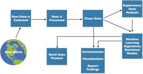
Data science is a multidisciplinary blend of data inference, algorithm development, and technology in order to solve analytically complex problems.

 

Understanding the problem

The sinking of the RMS Titanic is one of the most infamous shipwrecks in history.  On April 15, 1912, during her maiden voyage, the Titanic sank after colliding with an   iceberg, killing 1502 out of 2224 passengers and crew. One of the reasons that the shipwreck led to such loss of life was that there were not enough lifeboats for the passengers and crew. Although there was some element of luck involved in surviving the sinking, some groups of people were more likely to survive than others, such as women, children, and the upper-class.

Our aim is to predict the survival of passengers(whether they survive or perish) based on available features. This is a Binary classification: Supervised learning problem where we have to train a model to labeled outcome data(training set) and use this trained model to predict outcomes of test set.

 

Download the three data files from the data Section and read the Data Description carefully.

Data description:
The training set is used to build our machine learning models. For the training set, the outcome is already provided for each passenger. Our model will be based on “features” like passengers’ gender and class.
The test set should be used to see how well our model performs on unseen data. For the test set, the outcome is not provided and it’s our job to predict these outcomes.
There’s also a gender_submission csv file,which is a set of predictions that assume all and only female passengers survive, as an example of what a submission file should look like.

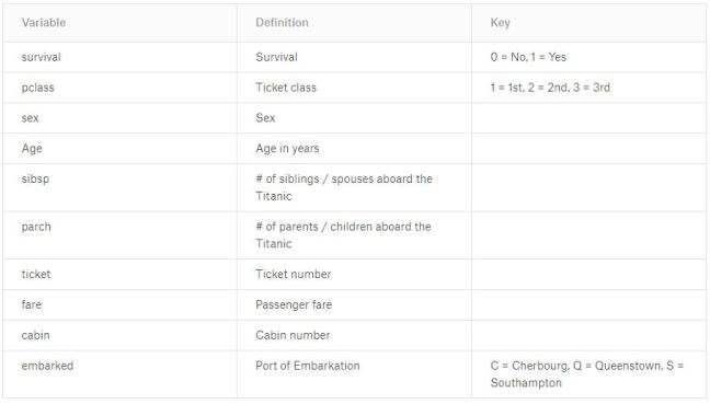
Survived: This is the outcome variable which is only present in the training set.
0 = No (perished)
1 = Yes (survived)

 

Pick a programming language(R or Python)
I am going to use R for this problem and if you haven’t used R at all, please go through this article(Getting started with R).

Open R studio and get started

#remove everything present in the working environment. 
rm(list =ls()) 
cat("\14") #clears console

#To install packages simply type install.packages("packageName")
install.packages("package name") 
#library loads installed packages  
library(ggplot2)  #Data Visualisations
library(randomForest)

After installing and loading packages we will set our working directory

#set working directory 
setwd("D:\\Projects\\Titanic") #specify path where you have your data

 

Import train and test csv files

# read.csv reads a file in table format and creates a data frame from it 
# the default for stringsAsFactors is true, as we do not wish to convert character vectors to factors we make it false 
train <- read.csv("train.csv", stringsAsFactors = FALSE)  
test <- read.csv("test.csv",stringsAsFactors = FALSE)

Once the data is imported view the data

#view data 
View(train) 
head(train) 
head(test)

Now we are going to combine these both test and train data frames, but for combining data frames by ‘rbind’ i.e row bind the numbers of columns of arguments must match. hence we add “survived” column to the test data frame and fill it with NA’s.

#adding survived variable to test set 
test$Survived <- NA
#combining both test and train dataframe by rows
fullset <- rbind(train,test)

---

Exploratory analysis

• Check for data, how it is scattered?
• Dataset dimensions
• Variable names
• How many unique values are there in each row?
• Outliers
• Missing values

 

#get the basic structure and description of fullset  
str(fullset) 
'data.frame': 1309 obs. of  12 variables:  
$ PassengerId: int  1 2 3 4 5 6 7 8 9 10 ...  
$ Survived   : int  0 1 1 1 0 0 0 0 1 1 ...  
$ Pclass     : int  3 1 3 1 3 3 1 3 3 2 ...  
$ Name       : chr  "Braund, Mr. Owen Harris" "Cumings, Mrs. John Bradley (Florence Briggs Thayer)" "Heikkinen, Miss. Laina" "Futrelle, Mrs. Jacques Heath (Lily May Peel)" ...  
$ Sex        : chr  "male" "female" "female" "female" ...  
$ Age        : num  22 38 26 35 35 NA 54 2 27 14 ...  
$ SibSp      : int  1 1 0 1 0 0 0 3 0 1 ...  
$ Parch      : int  0 0 0 0 0 0 0 1 2 0 ...  
$ Ticket     : chr  "A/5 21171" "PC 17599" "STON/O2. 3101282" "113803" ...  
$ Fare       : num  7.25 71.28 7.92 53.1 8.05 ...  
$ Cabin      : chr  "" "C85" "" "C123" ...  
$ Embarked   : chr  "S" "C" "S" "S" ... 
# study the variables

summary(fullset)   #check mean, median and number of NA's for each variable

 

Understanding the features and checking what role they play in survival.
We have 1309 observations(rows) and 12 Variables(columns). PassengerId is just a serial number and is not at all useful to us. Survived is the outcome or the dependent variable. Age, Fare, Embarked and Cabin all have missing values which we will deal with later.

 

Pclass shows which class a passenger is travelling, with 1st class being the highest ranked class. So it is a factor having three levels and it does not have any missing values.

fullset$Pclass <- as.factor(fullset$Pclass) #converting to factor
 #Visualizing Pclass 
ggplot(fullset[1:891,], aes(x = Pclass, fill = factor(Survived))) +   
  geom_bar() +  
  ggtitle("Impact of Class on Survival")

 

 

Sex: Females were more likely to survive, let’s check that out.

fullset$Sex <- as.factor(fullset$Sex) summary(fullset$Sex)
female male 
 466   843  
ggplot(fullset[1:891,], aes(x = Sex, fill = factor(Survived))) +  
 geom_bar() + 
 ggtitle("Do females have higher survival rate?")

Whoa! certainly a lot of females have survived as compared to the males. We have to dig deeper to understand if there’s is any other relation.

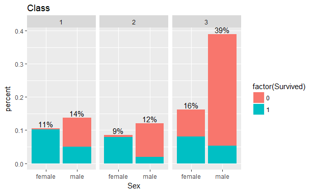
It looks like almost all the females from 1st and 2nd class Survive but females in the third class have only 50% chances.

---

Feature Engineering

Feature engineering is the process of transforming raw data into features that better represent the underlying problem to the predictive models, resulting in improved model accuracy on unseen data.

It is the science of extracting more information from existing data. This newly extracted information can be used as input to our prediction model. So,  better the features that you prepare and choose, the better the results you will achieve.

Creating New derived variables.

Interpreting the Name

head(fullset$Name)

[1] "Braund, Mr. Owen Harris"                            
[2] "Cumings, Mrs. John Bradley (Florence Briggs Thayer)"
[3] "Heikkinen, Miss. Laina"                             
[4] "Futrelle, Mrs. Jacques Heath (Lily May Peel)"       
[5] "Allen, Mr. William Henry"                           
[6] "Moran, Mr. James"

#creating new title variable from Name  
fullset$Title <- sapply(fullset$Name,FUN = function(x){strsplit(x,"[,.]")[[1]][2]}) 
fullset$Title <- sub(' ', '', fullset$Title) 
fullset$Title <- as.factor(fullset$Title) 

summary(fullset$Title)

Capt Col Don Dona Dr Jonkheer 
 1    4   1   1   8   1 
 Lady Major Master Miss Mlle Mme 
 1     2     61    260    2  1 
 Mr  Mrs  Ms Rev Sir theCountess 
 757 197  2   8   1   1

table(fullset$Sex,fullset$Title)

# There are many titles having less frequency and they can be grouped.
fullset$Title <- as.character(fullset$Title) 
fullset$Title[fullset$Title %in% c("Mlle","Ms")] <- "Miss" 
fullset$Title[fullset$Title == "Mme"] <- "Mrs" 
fullset$Title[fullset$Title %in% c( "Don", "Sir", "Jonkheer","Rev","Dr")] <- "Sir" 
fullset$Title[fullset$Title %in% c("Dona", "Lady", "the Countess")] <- "Lady" 
fullset$Title[fullset$Title %in% c("Capt","Col", "Major")] <- "Officer" 
fullset$Title <- as.factor(fullset$Title) 

summary(fullset$Title) 
Lady Master Miss Mr Mrs Officer Sir 
 3 61 264 757 198 7 19 


ggplot(fullset[1:891,], aes(x = Age)) +  
 geom_histogram(aes(y = ..density.., color = Title, fill = Title), alpha = 0.4, position = "identity") + 
  geom_density(aes(color = Title), size =1)

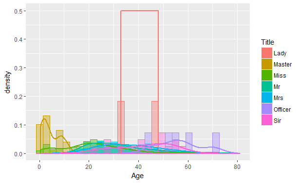
There are 7 different titles and every title is spread over some particular age range. ‘Master’ is spread over 0 to 18 and ‘Mr’ from about 18 to 65. The title ‘Miss’ i.e unmarried women and girls have age range of 0 to 65, here I would like to create one more title as Miss2 where we will have unmarried females(Miss) whose age is less than 18.  But as the Age variable has missing values we have to impute those first.

Family size can take a major role in our prediction. The family variable can be created by simply adding the number of siblings/spouses, parents/children and the that person himself.

fullset$FamSize <- fullset$SibSp + fullset$Parch + 1

ggplot(fullset[1:891,], aes(x = FamSize, fill = factor(Survived))) +
 geom_bar(stat='count', position='dodge') +
 scale_x_continuous(breaks=c(1:11)) +
 labs(x = 'Family Size')+ ggtitle("Family")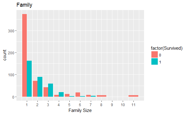

We will group these families according to their family size.

fullset$FamGroup[fullset$FamSize == 1] <- 'Individual' 
fullset$FamGroup[fullset$FamSize < 5 & fullset$FamSize > 1] <- 'small' 
fullset$FamGroup[fullset$FamSize > 4] <- 'large' 
fullset$FamGroup <- as.factor(fullset$FamGroup)

 

 

Missing value Imputation

Fare

sum(is.na(fullset$Fare))
[1] 1
 which(is.na(fullset$Fare))
[1] 1044
 #Imputing median Fare value of Pclass = 3 and Emabrked = S 
fullset$Fare[1044] <- median(fullset[fullset$Pclass == '3' & fullset$Embarked == 'S', ]$Fare, na.rm = TRUE)

 

Many Passengers have same Ticket numbers suggesting that they were travelling together and their fare is addition of the number of people travelling on a same ticket. So we find out fare per person and create a new variable Fare2 by dividing the fare for similar tickets.

n <- data.frame(table(fullset$Ticket))
fullset <- merge(fullset,n, by.x="Ticket", by.y="Var1", x.all=T) # Assign the frequency of each ticket appearance
fullset$Fare2 <- fullset$Fare / fullset$Freq

fullset <- fullset[order(fullset$PassengerId),]

 

Cabin:

which(fullset$Cabin == '')

It has more than a thousand missing values and hence we will ignore the cabin column.

 

Embarked

which(fullset$Embarked == '') 
fullset[c(62,830),]

seems like both ladies are from 1st class and have paid 40 bucks. Lets check out who else is paying 40 and is from 1st class.

fullset$Embarked <- as.factor(fullset$Embarked) 
fullset[fullset$Fare2 >= 39 & fullset$Fare2 <= 41 & fullset$Pclass == 1,]

summary(fullset[fullset$Fare2 >= 39 & fullset$Fare2 <= 41 & fullset$Pclass == 1,"Embarked"])
  C  Q  S 
 11  0  1 

so these females must have embarked from Cherbourg

fullset$Embarked <- as.character(fullset$Embarked) 
fullset$Embarked[fullset$Embarked %in% c("","")] <- "C" 
fullset$Embarked <- as.factor(fullset$Embarked)

 

Age

sum(is.na(fullset$Age)) 
[1] 263

we are going to treat these 263 missing age values according to the median of their title.

title.age <- aggregate(fullset$Age,by = list(fullset$Title), FUN = function(x) median(x, na.rm = T)) fullset[is.na(fullset$Age), "Age"] <- apply(fullset[is.na(fullset$Age), ] , 1, function(x) title.age[title.age[, 1]==x["Title"], 2])

sum(is.na(fullset$Age))
[1] 0

ggplot(fullset[1:891,], aes(Age, fill = factor(Survived))) +  
 facet_grid(.~Sex) + 
 geom_dotplot(binwidth = 2)

creating Miss2 level in Title

fullset$Title <- as.character(fullset$Title) 
fullset[fullset$Sex == "female" & fullset$Age < 18,"Title"] <- "Miss2" 
fullset$Title <- as.factor(fullset$Title)

summary(fullset$Title)
 Lady Master Miss Miss2  Mr  Mrs Officer Sir 
  3     61    197   72  757  193    7    19 

 

It was their saying “Women and Children first”, so we make a new variable to specify whether a person is Minor or Adult.

fullset$isMinor[fullset$Age < 18] <- 'Minor' 
fullset$isMinor[fullset$Age >= 18] <- 'Adult' 
fullset$isMinor <- as.factor(fullset$isMinor)
fullset$Survived <- as.factor(fullset$Survived) 

---

Splitting data into training and test set

#We will again split the data to train and test set
train <- fullset[1:891,] 
test <- fullset[892:1309,]

 

Modelling

Ensemble methods use multiple learning models to gain better predictive results — in the case of a Random Forest, the model creates an entire forest of random uncorrelated decision trees to arrive at the best possible answer.Random Forests grows many classification trees. To classify a new object from an input vector, put the input vector down each of the trees in the forest. Each tree gives a classification, and we say the tree “votes” for that class. The forest chooses the classification having the most votes (over all the trees in the forest). We have chosen Random Forest algorithm as it works well with a mixture of numerical as well as categorical features.

 

When the training set for the current tree is drawn by sampling with replacement, about one-third of the cases are left out of the sample. This oob (out-of-bag) data is used to get a running unbiased estimate of the classification error as trees are added to the forest. It is also used to get estimates of variable importance. After each tree is built, all of the data are run down the tree, and proximities are computed for each pair of cases.

 

set.seed(786) # to get a reproducible random result.
model <- randomForest(factor(Survived) ~ Pclass + Fare + Title + Embarked + FamGroup + Sex + isMinor,
 data = train, importance = TRUE, ntree = 1000,mtry=2)
#ntree is number of trees to grow. 
#mtry is number of variables randomly sampled as candidates at each split.
#importance: importance of predictors

model
OOB estimate of error rate: 16.61%
Confusion matrix:
   0    1  class.error
0 505  44  0.08014572
1 104 238  0.30409357

varImpPlot(model) 

importance(model)

           0        1       MeanDecreaseAccuracy   MeanDecreaseGini
Pclass  32.46637  39.83024         49.19026            32.134932
Fare    23.89813  32.03873         41.38793            49.645995
Title   35.37802  35.96153         42.29162            76.865798
Embarked 6.20003  19.48776         20.4500             8.541241
FamGroup 28.74773 21.10494         39.97892            22.083775
Sex      36.74055 27.92392         39.12383            54.886723
isMinor 10.58379  16.16442         19.98419            5.315404

 

Finally our model is trained, and now its time to apply this model to test data and predict result.

#predicting on test data
prediction <- predict(model,test) 
#creating a submission data frame of required format
submission <- data.frame(PassengerID = test$PassengerId, Survived = prediction) 
#write a csv output file
write.csv(submission, file = 'Submission.csv', row.names = F)

 

Congratulations! you’ve just made your first kaggle submission with an amazing accuracy and you are now in top 3% on the leaderboard.

we have made a simple yet effective model, which can obviously be improved further. Try on your own to play with features and different algorithms which will certainly help you learn many things.

 

 

I hope you found this tutorial useful and hope you to participate in more advanced kaggle competitions.

The code can be found on Github

Thank you for taking the time to read this tutorial. Any feedback and suggestions are highly appreciated.